KV Caching
core logic (matrix dimensions):
goal: generate one new token at a time. input: most recent token, shape [b, 1, n]. b: batch size, n: embedding dim, t: current sequence length.
step-by-step for token t+1:
projection:
input [b, 1, n] × weight matrix W_qkv [b, n, 3n] → [b, 1, 3n]
split into:
q_new [b, 1, n]
k_new [b, 1, n]
v_new [b, 1, n]
use cache:
retrieve K_cache [b, t, n], V_cache [b, t, n]
append new:
K_total = concat(K_cache, k_new) → [b, t+1, n]
V_total = concat(V_cache, v_new) → [b, t+1, n]
attention calculation:
scores: q_new @ K_total^T → [b, 1, t+1]
weights: softmax(scores / sqrt(n)) → [b, 1, t+1]
output: weights @ V_total → [b, 1, n]
result: output [b, 1, n], passed to next layer for next token prediction.
if you ever forget why we can store k and v as cache and how is it equivalent to doing fully, just remember the row matrix multiplication , you will realize
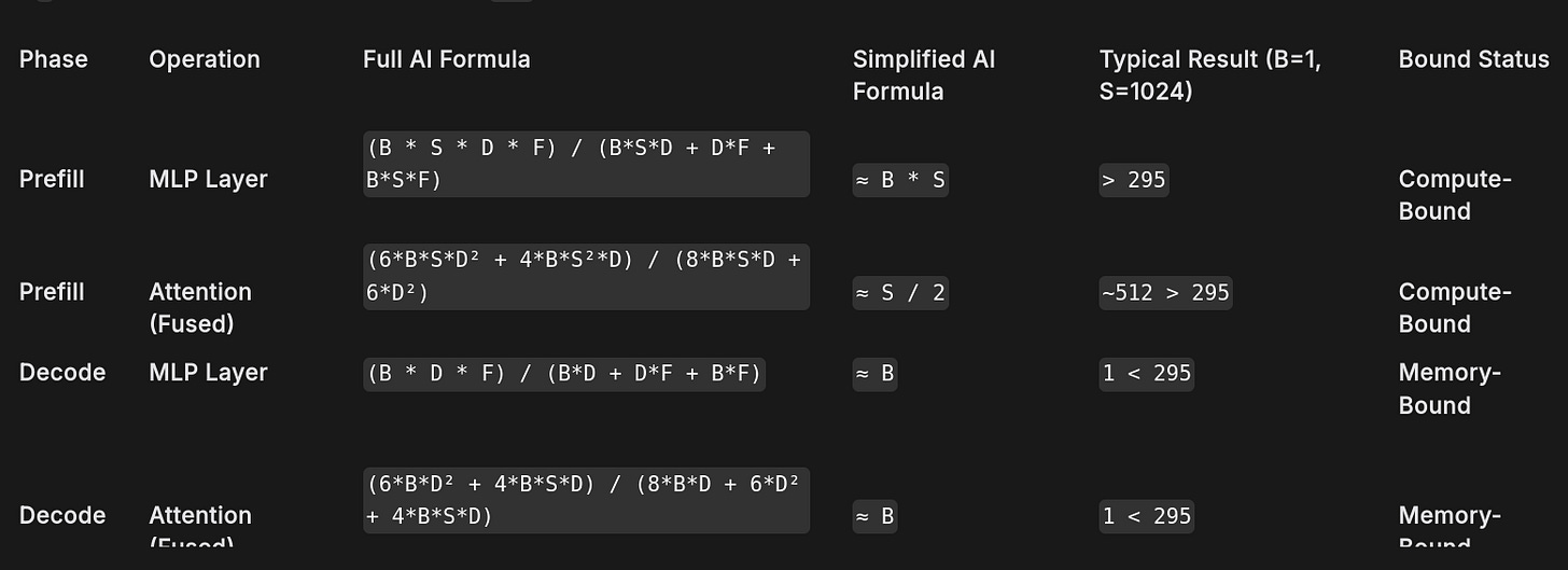
Arithmetic Intensity Analysis of Transformer Operations (on NVIDIA H100)
Machine Balance (AI_knee): ~295 FLOPs / Byte
If AI > 295: Compute-Bound (Limited by 989 TFLOP/s)
If AI < 295: Memory-Bound (Limited by 3.35 TB/s)
B: Batch Size
S: Sequence Length
D: Model Hidden Dimension
F: MLP Intermediate Dimension (typically ~4D)
kv cache memory calculation
calculation per layer:
memory for keys: b × s × h × d_k × 2 bytes
memory for values: b × s × h × d_k × 2 bytes
total per layer: b × s × h × 2 × d_k × 2 bytes = b × s × 2 × d × 2 bytes (since h × d_k = d)
total for entire model:
- kv cache size (bytes) = b × s × l × 2 × d × 2
example: llama 2 13b
l = 40 layers, d = 5120, b = 1, s = 4096
cache size = 1 × 4096 × 40 × 2 × 5120 × 2 = 3,355,443,200 bytes ≈ 3.36 gb
this is in addition to ~26 gb for model weights
kv cache size is proportional to the number of key and value vectors stored. standard mha is inefficient.
revisiting multi-head attention (mha)
structure: in mha, the model’s hidden dimension d is split among n attention heads. each head operates independently with its own query, key, and value projection weights (w_q, w_k, w_v).
implication for kv cache: if a model has n query heads, it also has n key heads and n value heads. for every token, we must compute and store n distinct key vectors and n distinct value vectors.
visualization: query heads: [q1] [q2] [q3] [q4] [q5] [q6] [q7] [q8] key heads: [k1] [k2] [k3] [k4] [k5] [k6] [k7] [k8] value heads: [v1] [v2] [v3] [v4] [v5] [v6] [v7] [v8]
the number of k/v heads is equal to the number of q heads.
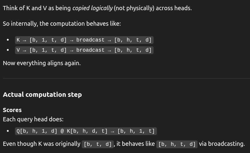
multi-query attention (mqa) mqa is based on a simple observation: the model might not need the full expressive power of n distinct key and value heads.
structure: mqa maintains n query heads but uses only a single key head and a single value head.
these single k/v heads are shared across all n query heads. implication for kv cache: for every token, we compute n q vectors, but only one k vector and one v vector.
visualization: query heads: [q1] [q2] [q3] [q4] [q5] [q6] [q7] [q8] key head: +-------------------[ k ]-------------------+ value head: +-------------------[ v ]-------------------+
benefit: the size of the kv cache is reduced by a factor of n (the number of heads). for a model with 40 heads, this is a 40x reduction in cache size and a 40x reduction in the amount of data that needs to be read from hbm during the decode step’s attention calculation. this directly improves tpot (time-per-output-token).
grouped-query attention (gqa) gqa is an interpolation between the extremes of mha and mqa. it recognizes that while mqa offers huge savings, the quality degradation from sharing a single k/v head might be too severe.
structure: gqa maintains n query heads, but groups them. each group of g query heads shares a single key/value head pair. the total number of k/v heads is n/g. implication for kv cache: it offers a tunable trade-off.
if g=1, you have n/1 = n k/v heads, which is identical to mha. if g=n, you have n/n = 1 k/v head, which is identical to mqa.
visualization (n=8, g=4): query heads: [q1] [q2] [q3] [q4] | [q5] [q6] [q7] [q8] key heads: +------[ k1 ]------+ | +------[ k2 ]------+ value heads: +------[ v1 ]------+ | +------[ v2 ]------+
benefit: reduces kv cache size by a factor of g. llama 2 models, for instance, use gqa to manage their kv cache size while maintaining high quality.
multi-head latent attention (mla) mla (used in the deepseek-v2 model) takes a different approach to dimension reduction. instead of reducing the number of k/v heads, it reduces the dimension of each k/v vector. structure: mla projects the full-dimension key and value vectors (n_h_d_k) down to a much smaller compressed or “latent” dimension, c. example (deepseek-v2): full k/v dimension: 16384multi-head latent attention (mla) reduces kv cache size by compressing the dimension of each key and value vector, rather than reducing the number of heads. instead of storing full-dimensional k/v vectors (nhd_k), mla projects them down to a much smaller latent dimension c using a compression matrix. for example, in deepseek-v2, the full k/v dimension is 16384, which is compressed to 512, giving a 32x reduction in cache size.
the data flow for mla is as follows:
input: token embedding x, shape (1, d)
k-projection: x is multiplied by the key weight matrix w_k to get the full-dimensional key k_full (1, d)
compression: k_full is then multiplied by a new compression matrix w_compress (d, c) to get the compressed key k_latent (1, c)
storage: only k_latent is stored in the kv cache; k_full is discarded
attention: when a new query q_full is generated, it is also compressed using w_compress to get q_latent (1, c)
scores: attention scores are computed in the latent space: q_latent @ k_cache_latent^t
decompression: the attention output (c-dimensional) is projected back to the full model dimension d using a decompression matrix w_decompress (c, d)
a wrinkle is that compression can interfere with positional encodings like rope, which work on the full-dimensional vectors. to handle this, deepseek-v2 adds back 64 dimensions, making the final latent dimension 576. this allows efficient cache storage while preserving the ability to use advanced positional encodings. compressed latent dimension c: 512
cross-layer attention (cla) the idea: gqa shares key/value vectors across heads in the same layer. cla extends this by sharing key/value vectors across multiple consecutive layers. mechanism:
layer 10 computes and caches its own k and v vectors.
layer 11 skips k/v computation and reuses the cache from layer 10 for its attention.
layer 12 does the same. benefit: memory savings are substantial—sharing one kv cache across 3 layers reduces memory by 3x. trade-off: model loses expressive power, as layers share less specialized information. must be trained from scratch with this architecture.
local attention (sliding window attention) the idea: for many tasks, only the local context matters. long-range dependencies are often negligible. mechanism: each token only attends to a fixed window of recent tokens (e.g., last 512 or 4096). visualization:
full attention: token 8000 attends to all previous tokens.
local attention: token 8000 attends only to last 512 tokens. benefit - compute: q @ k^t matrix multiplication is much smaller, speeding up prefill for long sequences. benefit - cache: kv cache size is fixed (independent of sequence length). oldest tokens are evicted as new ones arrive, enabling infinite sequences with small cache. cache size (local): b × w × l × 2 × d × 2 problem: model becomes short-sighted—cannot access distant context, hurting tasks needing long-range dependencies. solution - hybrid layers: most layers use local attention, but every nth layer uses full attention. balances efficiency with long-range coherence.
tell me what would would be the the dimensions of Value, and how
the static batching problem
static batching (batched scheduling):
inference server collects b user requests, pads them to the length of the longest request, and processes them as one dense tensor.
processing starts only when batch is full or timeout reached.
example: three requests:
a: “the cat sat on the” (5)
b: “summarize this article” (4)
c: “translate to french: hello” (3)
padded batch:
[ the, cat, sat, on, the ] [ summ, this, article, p, p ] [ tran, to, french, hello, p ]
forms a (b=3, s=5) tensor for efficient gpu processing.
inefficiencies of static batching:
a. throughput inefficiency (padding):
gpu computes on padding tokens—wasted computation.
in example, 3/15 slots (20%) are padding. real workloads often see 50–70% waste.
reduces max throughput; wastes compute and kv cache memory.
b. latency inefficiency (head-of-line blocking):
short, fast requests wait for longer ones in the queue.
requests arriving early wait for batch to fill or for long requests to finish.
consequences:
high time-to-first-token (ttft): early requests delayed by 100–500ms.
poor fairness: fast requests wait behind slow ones, hurting user experience.
How padding really works
the attention mask
the attention mask is the key mechanism that prevents the model from attending to padding tokens.
before softmax, a mask matrix is added to the attention scores (q @ k^t).
mask contains 0 where attention is allowed, and a large negative number (e.g., -1e9) at padding positions.
after softmax, scores for padding positions become effectively zero.
result: no token attends to padding tokens—they are invisible to attention.
masking during loss
example: batch of two sequences
sequence 1: [the, cat, sat, ] (length 4)
sequence 2: [hello, world, , ] (length 4 after padding)
prediction targets (y values)
for each input, the target is the next token in its own sequence.
after , there is no meaningful target—the sequence is over.
why masked loss is necessary
the model produces logits at every position, even after and at .
if we don’t mask loss at these positions, the model would be forced to predict something after the sequence ends.
this would teach nonsense patterns, corrupting language understanding.
solution: gradients for and tokens are set to zero.
these positions are ignored during training.
the network does not learn from them, preserving correct language structure.
note in static batching you can not do prefill and decode together, because then the padding for the decode tokens would become very very massive
Continuous batching
instead of looking it like we will wait for some pre-fixed batch of user requests, what we do is we see it as a per token generation or per forward pass iteration. for one forward pass the batch and sequence length does not change but for another forward pass they might change, based on the user request. in that single forward pass we want have many requests of type both prefill and decode. the decode type will have sequence length of 1 only but the prefill one can have varying sequence lengths so the way we are looking at it now even doing a forward pass is impossible
you can not have (batch , changing not constant sequence, dimension) size fo a matrix and do a matrix multiplication. so what we do instead is multiply the batch and sequence (or add all the sequence).
suppose there is a prefill request of 500 tokens and 4 decode request so our matrix will become of size (504, n) and multiplying it with a (n, 4n) matrix is now possible
now lets look at the attention mechanism.
you would have notices that we can generate k q v vectors of each token in parallel now also that is not an issue but
q * k ^ Transpose. this operation is hard to do because the last dimension of k keeps changing for both decode and prefill so we can not batch them. so we will have to do them in parallel but we will have to write a custom cuda kernel to do this efficiently.
now while writing the custom cuda kernel there is a issue, to solve which we introduce
paged attention
without pagedattention, each new request requires a contiguous block of gpu vram for its full kv cache:
request a (max_len=1024): allocate 1024-token block
request b (max_len=2048): allocate 2048-token block
request c (max_len=1024): allocate another 1024-token block
this causes two major problems:
internal fragmentation:
- if request a only uses 50 tokens, 974 token-slots are wasted, even though they’re allocated.
external fragmentation:
when request b finishes, its 2048-token block is freed.
a new request d needs 2049 tokens. even if total free memory is enough, if no single contiguous block is large enough, the request fails.
this fragmentation makes memory management inefficient and scheduler complex.
pagedattention: the solution
pagedattention applies the idea of paging from os virtual memory:
physical memory: gpu kv cache is split into many small, fixed-size blocks (pages), e.g., 16 tokens per block.
logical view: each sequence sees its kv cache as a continuous sequence.
page table: for each request, a lookup table maps logical blocks to physical blocks in memory.
this allows flexible allocation, reduces fragmentation, and makes memory usage much more efficient.
Speculative Sampling
step 1: drafting (fast & sequential)
a small, fast draft model (m_draft) runs autoregressively and generates k candidate tokens.
example: draft predicts [”the”, “quick”, “brown”, “fox”]. this is fast due to the model’s small size.
step 2: verification (fast & parallel)
the large target model (m_target) takes the original context plus the entire draft as input.
one forward pass produces probability distributions (logits) for each draft position.
step 3: acceptance/rejection (rejection sampling)
compare draft predictions with target model’s probabilities token by token.
token 1 (”the”): if p_target(”the”) is high, accept.
token 2 (”quick”): if previous token accepted, check p_target(”quick” | “the”). if high, accept.
token 3 (”brown”): if target prefers “red”, reject “brown”.
chain breaks: any rejection discards the rest of the draft.
step 4: correction and resumption
keep accepted tokens (e.g., [”the”, “quick”]).
at the rejection point, sample a corrected token from target model’s logits (e.g., “red”).
resume generation from the corrected token. draft model generates a new draft from there.
performance gain
one draft and one verification step can yield multiple tokens.
speedup depends on acceptance rate: better draft models = longer accepted sequences = greater speedup.
method is lossless: final sequence matches target model’s distribution exactly.
not an approximation—just a faster generation method.
Distillation
inputs: standard text dataset (e.g., “the quick brown...”).
forward pass (student):
text is fed into the student model.
produces logits for next token (e.g., fox: 5.0, dog: 2.0, car: -10.0).
forward pass (teacher):
same text is fed into the frozen teacher model.
produces its own logits (e.g., fox: 10.0, dog: 8.0, car: -20.0).
loss function (the “training” part):
standard supervised learning: loss checks if model predicted the correct single word.
distillation: loss (kl-divergence) checks if student’s probability distribution matches teacher’s.
this is “curve fitting.”
step 1: softmax with temperature
divide logits by temperature t before softmax.
high t smooths the distribution, making small probabilities more visible.
p_student = softmax(student_logits / t)
p_teacher = softmax(teacher_logits / t)
step 2: calculate divergence
- loss = kl_divergence(p_teacher, p_student)
step 3: backpropagation
gradients of loss are calculated w.r.t. student’s weights.
optimizer updates student to match teacher’s output curve.
teacher weights remain frozen.
in quantization weights are stored in quantized manner but to do calculations they are converted to bf16
also pruning is removing some layers based on how active they are in a sample dataset